himawari: satellite wind-flow analytics

A data-engineering project built with Parit Vacharaskunee. It takes raw scientific data from the NOAA Himawari-8/9 bucket on AWS S3 Open Data and turns it into wind-flow maps of Thailand, a wind forecast, and a dashboard that replays it all as if it were live.

Stack: Apache Airflow · Kafka (Redpanda) · MinIO · ClickHouse · PostgreSQL · PyTorch · Streamlit · Docker Compose

Pipeline

1. Ingestion. An Airflow DAG polls the S3 bucket for new files and pushes a metadata “ticket” for each one into Kafka (Redpanda). Consumers pick the tickets up independently, so ingestion, processing and analytics are decoupled. We target Band 13 (infrared, for cloud-top temperature and storm cores) and Band 08 (water vapour, for high-altitude motion).
2. Image processing. Satpy calibrates the raw AHI files, and Pyresample reprojects them onto a 0.05° grid over Southeast Asia. From there we produce thermal heatmaps and true-colour RGB composites, with gray-world white balancing and sRGB gamma correction.
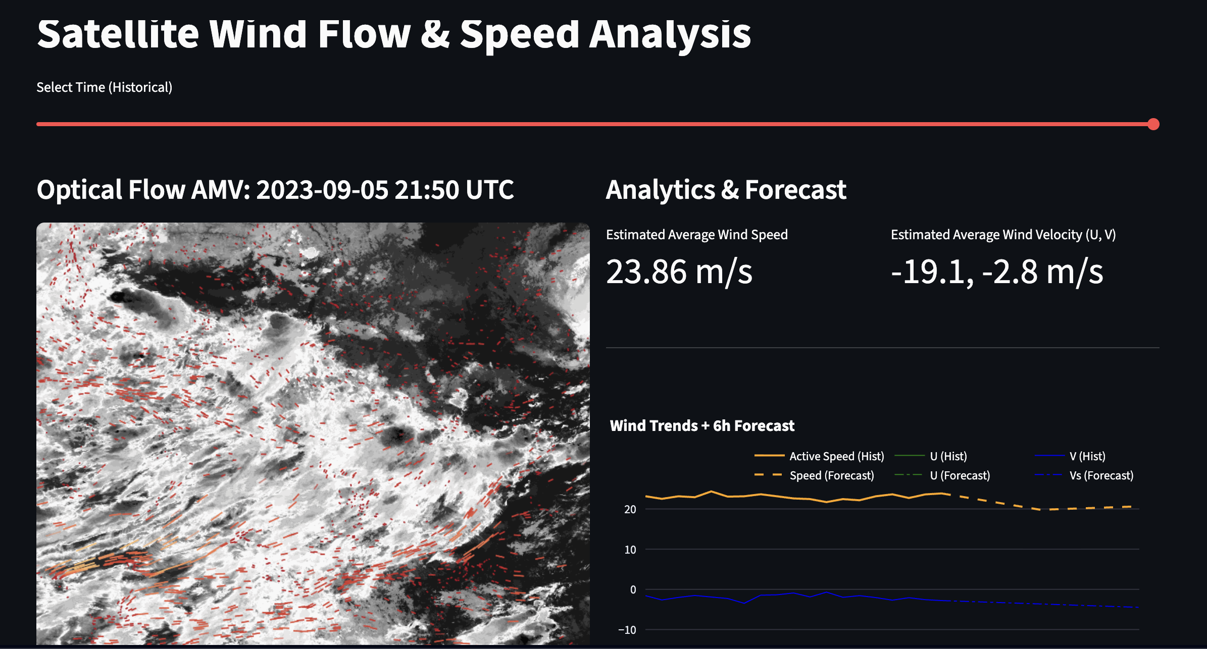
3. Wind vectors. Farnebäck optical flow compares consecutive frames to get per-pixel displacement, which gives atmospheric motion vectors (AMVs).
4. Storage. Animated wind-flow visuals go to MinIO (S3-compatible). Aggregated metrics such as max speed and average U/V velocity go into ClickHouse (MergeTree), where weeks of data can be queried in milliseconds.
5. Forecasting. An LSTM trained on the derived U/V sequences predicts wind intensity for the next six hours.
6. Dashboard. A Streamlit app has a time slider for scrubbing through imagery, actual-vs-forecast charts, and wind streaks animated over the map.

What was hard

• Ingestion speed. Downloading and processing one day of 10-minute data took about 7 hours, because the files are large and the bucket is in a distant region. We switched to hourly timestamps so we could ingest more than a year of data.
• Memory. High-resolution RGB composites kept running out of memory during batch processing. Per-band processing and giving Docker 12 GB of RAM fixed it.
• Picking the motion algorithm. Our first attempt used phase cross-correlation on a grid of image tiles, and it was inaccurate. After reading Deriving AMVs from Geostationary Satellite Images Using Optical Flow Algorithm Based on Polynomial Expansion, we switched to Farnebäck optical flow, which gave far more stable vectors.